
Technical Project:
Statistics for Data Analysis using Excel
Disclaimer. Please access this case study from a computer. The formatting may be slightly off on mobile or tablet devices and could hinder your understanding of the content. As you scroll down, you’ll see sections with click-to-expand arrows that allow for a deeper dive into each section. After reading each section, please click the arrow again to reset the section. This project showcases my practical application and knowledge of Excel using statistics for data analysis. While this project accurately represents my work, it is not a standard analysis. We sourced the dataset from Kaggle.com, though some data was modified for demonstration purposes. This includes cleaning or standardizing fields and adding or removing records to illustrate technical concepts. Credit for the comprehensive statistics workflow in this project goes to Maven Analytics. It's also important to clarify that all numbers referring to monetary values, such as sales and ad spending, are in millions. This includes the coefficients, standard errors, and confidence intervals mentioned in the analysis.
Click the play button below to listen to this technical project!
Interested in working together?
Project Overview

Business Consulting & CO.
Business Intelligence Analysts who help organizations leverage data for strategic decision-making.
Introduction
Business Consulting & Co. is excited to announce our ongoing contract with global advertising agency Infinite Reach Advertising. Our analysts are responsible for providing data analysis to assist Infinite Reach's marketing team with strategic decision-making and to provide valuable support through our data analytics and business consulting expertise.
Objective
Utilize statistical analysis to assess the impact of influencer collaborations on sales generated from social media ad spending for Infinite Reach Advertising. This involves categorizing influencer collaborations by audience size (from Mega to Nano) to understand their effectiveness. Our goal is to evaluate past influencer program data performance, forecast future collaboration outcomes, and recommend recruitment adjustments to enhance advertising partnership outcomes. Ultimately, we aim to optimize advertising strategies, elevate performance, and provide significant value to clients and stakeholders.
My Role
As a marketing data analyst at Business Consulting & Co., I support the executive-level staff at Infinite Reach Advertising by gathering critical insights for their upcoming stakeholder meeting. My calendar has been blocked off in anticipation of the high volume of emails expected while Infinite Reach Advertising's dashboard is down. This ensures I can dedicate uninterrupted time to addressing urgent data analysis requests and providing timely updates to the executive team.
The Statistics Workflow
Statistics plays a crucial role in business intelligence by providing insights that aren't always recognizable through traditional means. By leveraging statistical techniques, businesses can make informed decisions, identify patterns and trends, forecast future outcomes, and optimize processes. Statistical methods also enable companies to extract valuable information from large datasets, understand customer behavior, evaluate the effectiveness of marketing campaigns, manage risks, and improve overall performance. Statistics empower businesses to better understand their operations, competitors, and market dynamics, enhancing strategic planning and driving success in a competitive environment.
Descriptive Statistics
Analyze data to understand its characteristics and patterns and guide further analysis.

Probability Distribution
Assess whether data fits a probability distribution that can accurately model the entire population.

Confidence Intervals
When data doesn't fit, we use the central limit theorem to estimate population parameters confidently.

Hypothesis Test
Apply the central limit theorem effectively to draw strong conclusions about the population.
Regression Analysis
Enhance prediction accuracy and insights by incorporating additional variables into the analysis.

Results:
How did all influencer types impact sales?
In summary, the combined results suggest a diverse and balanced influence of all influencer types on total sales, with a relatively uniform distribution of sales across different ranges.
The combined impact of all influencer types on total sales reflects a relatively balanced distribution, with each influencer type (Mega, Macro, Micro, and Nano) representing a similar proportion of the total influencers – ranging from approximately 24.54% to 25.33%. The distribution of sales across different sales ranges appears uniform, indicating no significant skewness (.07) or concentration of sales values in particular ranges.
For the total population, the mean sales amount is 192 million dollars, with a median of 189 million dollars. Approximately 68% of sales data falls within the range of 98.9M to 285.5M. The probability analysis indicates a 77% likelihood of sales figures being less than or equal to 260 million dollars based on the distribution of sales data.
Best Influencer Type?
Based on the comprehensive analysis of the entire dataset, Descriptive Statistics highlight Macro influencers as the most influential in driving sales, showcasing slightly higher mean and median sales figures compared to other influencer types. Conversely, Mega influencers exhibit comparatively lower mean and median sales figures. This suggests a potentially lesser impact on sales outcomes. Notably, Macro influencers stand out due to a combination of factors, including a lower margin of error, wider confidence interval, and similar variability in estimates compared to other influencer types. This positions them as a potentially more reliable and flexible choice for implementing influencer marketing strategies moving forward.
Based on the sample dataset, conversely, the worst influencer type in terms of influencing sales cannot be definitively determined from the hypothesis tests. This is because for the Mega, Macro, and Nano influencer types, the p-values are greater than the significance level of 0.15. Therefore, we fail to reject the null hypothesis for these influencer types, indicating that we do not have sufficient evidence to conclude that their average sales are significantly different from 192 million.
Recommendation:
Based on the findings conducted on each influencer type, individuals within each influencer category significantly contribute to sales outcomes. Therefore, we recommend conducting a future individual analysis on each influencer to understand their impact on sales performance better and tailor marketing strategies to leverage their effectiveness moving forward. This granular analysis will provide valuable insights into the specific influencers driving sales and allow for a more targeted and efficient allocation of resources in future marketing campaigns.

From: Jennifer Roberts
Subject: Descriptive Statistics
Hi Kristin,
The Director of Marketing for Infinite Reach Advertising, Samantha, is out on vacation. I will be covering for her. Unfortunately, Infinite Reach Advertising dashboard stopped working unexpectedly and is under maintenance until further notice. During this time, I'll require your help to gather insights from an Excel file for an upcoming important stakeholders meeting.
I can see influencer and sales data, but the data is overwhelming. I'm struggling to gain meaningful insights due to the sheer volume of numbers. I need to better understand sales generated as a result of the advertising efforts. I also need to know how many types of influencers we have worked with more clearly to assess potential tweaks to the influencer program.
Could you lend me a hand with this?
Thank you,
Jennifer Roberts
Key Objective
1. Create a frequency table for the “Influencer Types” variable.
2. Visualize sales data using a histogram.
-
Definition: Frequency represents the number of times a particular value or range of values occurs in a dataset. It provides information about the occurrence or prevalence of each value within the dataset.
-
Formula: It is calculated by dividing the frequency of a specific value or category by the total number of observations and expressing the result as a fraction or percentage.
Definition: Refers to the proportion or percentage of times a particular value or category occurs relative to the total number of observations or occurrences in a dataset.
-
Definition: Distribution refers to the manner in which data is spread out or dispersed across different values within a dataset. It provides insights into the range and variability of the data.
-
Definition: A histogram is a graphical representation of the frequency distribution of a dataset. It consists of a series of bars, where the height of each bar represents the frequency or relative frequency of corresponding data values. Histograms are used to visualize the distribution of numerical data and identify patterns or trends within the dataset.
Mega-Influencers:
Extremely large followings often exceeding millions of followers.
Frequency: 1,158
Relative Frequency: 25.33%
Macro-Influencers:
A large following, ranging from tens of thousands to millions of followers.
Frequency: 1,122
Relative Frequency: 24.54%
Micro-Influencers:
A smaller audience, from a few thousand to a hundred thousand followers.
Frequency: 1,153
Relative Frequency: 25.22%
Nano-Influencers:
A tiny niche audience of a few hundred to a few thousand followers on social media.
Frequency: 1,139
Relative Frequency: 24.91%
Summary: Based on the findings, we can see that each influencer type (Mega, Macro, Micro, and Nano) comprises a similar proportion of the total influencers, with relative frequencies ranging from approximately 24.54% to 25.33%. This indicates a relatively balanced distribution of influencer types within the dataset. It also suggests there is diversity in the sizes of influencers, with representation across various tiers (from mega to nano).
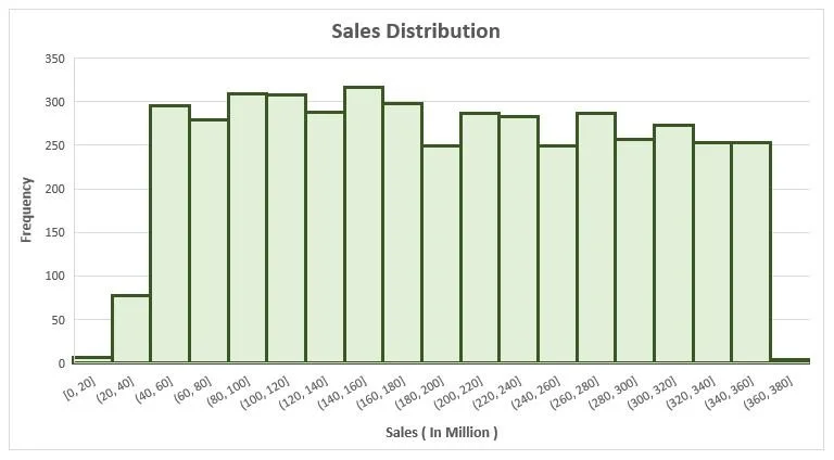
Histogram
The graph looks more uniform and suggests sales distribution is evenly spread across the different sales ranges. In other words, sales values have no significant skewness or concentration in particular ranges. This uniform distribution can help understand overall sales patterns and identify potential trends or data outliers.
From: Jennifer Roberts
Subject: Descriptive Statistics
Thanks for visualizing the sales data for me! It’s interesting to see the sales distribution. I wonder if Mega-influencers tend to do better than the other influencer types since it has the highest frequency.
Could you give me a quick summary about the total average sales and outline each influencer type average sales?
I’d appreciate it if you could interpret the results for me as well.
Thanks!
Jennifer Roberts
Key Objectives
1. Calculate the mean, median, mode, and skew for all sales and sales by each influencer type.
-
Excel Function: AVERAGE() or AVERAGEIFS()
Formula: Determined by dividing the sum of all values by the count of all observations.
Definition: The mean is the calculated "average" value in a set of numbers. This calculation exclusively applies to numerical variables and cannot be used with categorical data.
Additional Information: While the mean is often helpful in providing an estimated value, it's essential to supplement this with other descriptive statistics such as distribution, median, and mode to determine whether outliers influence the mean.
-
Excel Function: MEDIAN
Definition: The median is the "middle value" in a sorted set of numbers. The median is not sensitive to outliers. When there are two middle-ranked values, the median is the average of the two.
-
Excel Function: MODE.SNGL or MODE.MULT
Definition: The mode is the value that appears most frequently in a dataset. It represents the peak or the most common value in a distribution.
-
Excel Function: SKEW
Definition: Skew measures the asymmetry of the distribution of a dataset. A positive skew indicates a longer tail on the right side, while a negative skew indicates a longer tail on the left side. In a zero-skewed distribution, the mean and median are equal.
Mega-Influencers:
Mean: 190M
Median: 184M
Skew: .10
Macro-Influencers:
Mean: 195M
Median: 194M
Skew: .03
Micro-Influencers:
Mean: 192M
Median: 188M
Skew: .07
Nano-Influencers:
Mean: 192M
Median: 190M
Skew: .07
Total Population:
Mean: 192M
Median: 189M
Skew: .07
Summary: Macro influencers exhibit slightly higher mean and median sales figures. Conversely, Mega influencers show comparatively lower mean and median sales figures. This suggests a less significant influence. Notably, none of the influencer types display a mode, indicating a relatively even sales distribution across different values. The skew of all influencer types suggests a slight positive skewness, indicating a slightly higher frequency of sales figures toward the higher end of the distribution.
From: Jennifer Roberts
Subject: Descriptive Statistics
Interesting observation how mega influencers have the lowest mean and media sales but highest skew. I would like to investigate the sales data a bit further to understand more.
It would help if you could provide some sort of visual as well, especially since I’m taking this to the stakeholder meeting.
Thanks again!
Jennifer Roberts
Key Objectives
Calculate the range, interquartile range, and standard deviation for the sales variable by Influencer type.
Compare the sales data by influencer type by using a box and whicker plot.
-
Excel Function: MIN
Definition: The minimum is the smallest value in a dataset.
-
Excel Function: MAX
Definition: The maximum is the largest value in a dataset.
-
Formula: Maximum value minus the minimum value
Definition: The range is the difference between the maximum and minimum values in a dataset, representing the spread or variability of the data.
-
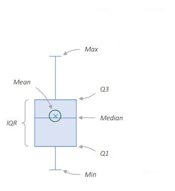
Definition: Box & Whisker plots, also known as boxplots, are graphical representations of the distribution of a dataset. They display key descriptive statistics such as the median, quartiles, and outliers in a compact and visually informative manner. The plot consists of a box, which spans the interquartile range (IQR) and contains the median, and "whiskers" extending from the box, which indicate variability outside the IQR.
-
Excel Function: VAR.P() or VAR.S()
Formula: The variance is calculated by averaging the squared differences between each data point and the mean of the dataset.
Definition: Variance measures the spread or dispersion of a dataset around its mean. It provides insight into the variability or diversity of the data points, with higher variance indicating greater dispersion from the mean.
-
Excel Function: QUARTILE.IN
Definition: The first quartile (Q1) is the value below which 25% of the data falls in a dataset, representing the lower quartile.
-
Excel Function: QUARTILE.IN
Definition: The third quartile (Q3) is the value below which 75% of the data falls in a dataset, representing the upper quartile.
-
Formula: Third quartile (Q3) minus first quartile (Q1)
Definition: The interquartile range (IQR) is the range of the middle 50% of the data, representing the spread of the central portion of the dataset.
-
Excel Function: STDEV.P() or STDEV.S()
Formula: The standard deviation is calculated as the square root of the variance.
Definition: The standard deviation is a measure of the amount of variation or dispersion in a dataset. It indicates the typical distance between each data point and the mean, with higher standard deviation values suggesting greater variability in the data.
-
Formula: Standard deviation divided by the mean
Definition: The coefficient of variation (CV) is a relative measure of dispersion that expresses the standard deviation as a percentage of the mean. It helps assess the consistency or variability of a dataset relative to its mean.
Box & Whisker Plot
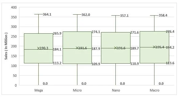
Mega-Influencers:
Variance: 8,561.19
Standard Deviation: 92.53
Coefficient of Variation: 49%
Macro-Influencers:
Variance: 8,588.75
Standard Deviation: 92.68
Coefficient of Variation: 47%
Micro-Influencers:
Variance: 8,908.58
Standard Deviation: 94.39
Coefficient of Variation: 49%
Nano-Influencers:
Variance: 8,761.04
Standard Deviation: 93.60
Coefficient of Variation: 49%
Total Population:
Variance: 8,709.04
Standard Deviation: 93.32
Coefficient of Variation: 49%
Summary: Despite differences in mean, median, and max sales, the interquartile ranges (IQR) are relatively consistent across influencer types. This suggests consistent variability in sales data, which was confirmed after calculations. A high variance and standard deviation number indicates that the data points are more spread out from the mean. A coefficient of variation of 0.49 means that the standard deviation is approximately 49% of the mean sales figure. This indicates a moderate level of relative variability in sales data across influencer types, where the dispersion of sales figures is around half of the mean value. Overall, Macro influencers appear to have the most significant influence on sales outcomes.
From: Jennifer Roberts
Subject: Probability Distributions
Is it possible you can make predictions based on sales data? We want to know the probability of sales being less than 260 million dollars.
We want to predict more realistic sales goals. What more info can you give us? Please provide an upper and lower range.
Thanks!
Jennifer Roberts
Key Objectives
Plot the distribution of sales to see if it resembles a bell curve.
Use excel formula NORM.INV to calculate the 25th and 75th percentile.
-
Excel Function: NORM.S.DIST
Formula: Z=(x-µ )/σ
Definition: The Z-score, also known as the standard score, measures the number of standard deviations a data point is from the mean of a dataset. It quantifies how far a data point deviates from the mean in terms of standard deviation units. A positive Z-score indicates that the data point is above the mean, while a negative Z-score indicates that it is below the mean.
-
Excel Function: NORM.DIST(True)
Definition: This calculates the probability of observing a value less than or equal to a specified value (Example: 260M) in a normal distribution with the given mean and standard deviation.
-
Excel Function: NORM.INV
Definition: This function calculates the value corresponding to a given probability in a standard normal distribution. In this case, it returns the value corresponding to the 25th percentile.
-
Excel Function: NORM.INV
Definition: This function calculates the value corresponding to a given probability in a standard normal distribution. In this case, it returns the value corresponding to the 75th percentile.
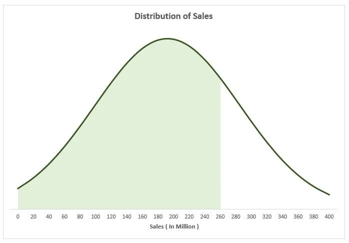
Probability of 260 Million in Sales
This outcome suggests there is a 77% probability that sales figures will be less than or equal to 260 million dollars based on the distribution of sales data. In other words, there's a high likelihood that sales will fall below or equal to 260 million dollars.
Lower Probability 25%: 129M
Upper Probability 75%: 255M
From: Jennifer Roberts
Subject: Probability Distributions
Could you please provide the percentages of sales that lie 1, 2, and 3 standard deviations from the mean? This analysis will help us understand the variability in our sales data and identify potential areas for improvement.
Jennifer Roberts
Key Objectives
Calculate the percentage of sales that lie 1, 2, and 3 standard deviations from the mean to see if the variable follows the empirical rule.
-
Definition: The Empirical Rule, also known as the 68-95-99.7 Rule or Three Sigma Rule, is a statistical guideline used to interpret data from a normal distribution. It states that approximately 68% of the data falls within one standard deviation of the mean, about 95% within two standard deviations, and nearly 99.7% within three standard deviations. This rule provides a quick way to assess the spread and distribution of data and identify potential outliers in a dataset.
-
Definition: In context of The Empirical Rule, "distribution" refers to the proportion or percentage of data points falling within specific ranges or intervals in a dataset. For example, when referring to the distribution of values between a lower and upper limit, it indicates the percentage of data points falling within that range. The values provided, such as 58.2%, 99.9%, and 100.0%, represent the proportion of data points falling within certain standard deviations from the mean, as per the empirical rule. Understanding the distribution helps in assessing the spread and concentration of data points, providing insights into the variability and patterns present within the dataset.
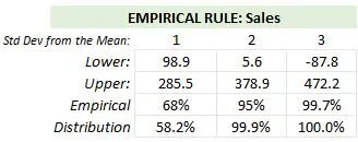
Empirical Rule for All Sales Data
One Standard Deviation: The mean is 192M for all sales data. Approximately 68% of the sales data falls, with values ranging from 98.9 to 285.5 million dollars. However, in our dataset, we observe that 58.2% of the actual sales data falls within this range, indicating some deviation from the expected distribution.
Two Standard Deviations: Approximately 95% of the data, with values ranging from 5.6 to 378.9 million dollars. In our dataset, we find that 99.9% of the actual sales data falls within this extended range, demonstrating a slightly higher concentration around the mean compared to the expected distribution.
Three Standard Deviations: the Empirical Rule suggests that approximately 99.7% of the data should fall, with values ranging from -87.8 to 472.2 million dollars. Interestingly, we find that 100.0% of the actual sales data falls within this range in our dataset, indicating a close alignment with the expected distribution.
From: Jennifer Roberts
Subject: Confidence Intervals
I keep thinking about the possibilities now that we know the sale averages from advertising follow a normal distribution.
Just out of curiosity though… what do sales look like in the top 10% for each influencer type? And how many standard deviations away from the mean (192M) would that be?
I’d appreciate it if you could interpret the results for me as well.
Jennifer Roberts
Key Objectives
Calculate the mean and known population.
Set a confidence level.
Calculate the margin of error; use the NORM.S.INV function to calculate the z-score (the population standard deviation (σ) is KNOWN) for the top 10%.
Set the limits for the confidence interval.
-
Definition: The lower limit of a confidence interval is the minimum value of the interval range, below which the true population parameter is not expected to fall with the specified level of confidence. It represents the lower bound of the estimated range and provides a measure of the precision or uncertainty associated with the estimate.
-
Definition: The upper limit of a confidence interval is the maximum value of the interval range, above which the true population parameter is not expected to fall with the specified level of confidence. It represents the upper bound of the estimated range and provides a measure of the precision or uncertainty associated with the estimate.
-
Definition: In statistics, the confidence level represents the degree of uncertainty or risk associated with a statistical estimate. It is often expressed as a percentage and indicates the probability that a confidence interval contains the true population parameter. For example, a 95% confidence level implies that if the sampling process were repeated multiple times, 95% of the resulting confidence intervals would contain the true population parameter. A higher confidence level indicates greater certainty but may result in wider confidence intervals. Commonly used confidence levels include 90%, 95%, and 99%.
-
Excel Function: NA
Formula: NA
Definition: In statistics, alpha (α) represents the significance level used in hypothesis testing. It is the probability of rejecting the null hypothesis when it is actually true. Typically, alpha is set at 0.05 or 0.01, indicating a 5% or 1% chance of making a Type I error, respectively.
-
Known as a false positive, occurs when the null hypothesis is incorrectly rejected when it is actually true. It represents the probability of concluding that there is a significant effect or difference when no such effect or difference exists in the population.
-
Definition: The standard error measures the variability or dispersion of sample means around the true population mean. It quantifies the accuracy of the sample statistic in estimating the population parameter. A smaller standard error indicates a more precise estimate, while a larger standard error suggests greater variability or uncertainty in the estimate.
-
Definition: The margin of error is a measure of the precision or uncertainty associated with estimating a population parameter from a sample statistic. It represents the maximum expected difference between the sample estimate and the true population value, given a certain level of confidence. The margin of error is typically expressed as a percentage or a fixed value.
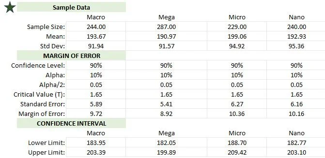
Mega Influencers:
Margin of Error: 4.47 million dollars
Our estimate of the mean sales for Mega influencers could vary by approximately ±4.47 million dollars from the true population mean.
Confidence Interval:
Lower Limit: 185.79 million dollars
Upper Limit: 194.74 million dollars
We are 90% confident that the true population mean falls between approximately 185.79 million dollars and 194.74 million dollars for Mega influencers.
Standard Error: 2.72 million dollars
The standard error of 2.72 million dollars indicates the variability in our estimate of the mean sales for Mega influencers.
Macro Influencers:
Margin of Error: 4.48 million dollars
This indicates that our estimate of the mean sales for Macro influencers could vary by approximately ±4.48 million dollars from the true population mean.
Confidence Interval:
Lower Limit: 190.96 million dollars
Upper Limit: 199.92 million dollars
We are 90% confident that the true population mean falls between approximately 190.96 million dollars and 199.92 million dollars for Macro influencers.
Standard Error: 2.72 million dollars
The standard error of 2.72 million dollars suggests the variability in our estimate of the mean sales for Macro influencers.
Micro Influencers:
Margin of Error: 4.57 million dollars
Our estimate of the mean sales for Micro influencers could vary by approximately ±4.57 million dollars from the true population mean.
Confidence Interval:
Lower Limit: 187.07 million dollars
Upper Limit: 196.21 million dollars
We are 90% confident that the true population mean falls between approximately 187.07 million dollars and 196.21 million dollars for Micro influencers.
Standard Error: 2.78 million dollars
The standard error of 2.78 million dollars suggests the variability in our estimate of the mean sales for Micro influencers.
Nano Influencers:
Margin of Error: 4.56 million dollars
Our estimate of the mean sales for Nano influencers could vary by approximately ±4.56 million dollars from the true population mean.
Confidence Interval:
Lower Limit: 187.04 million dollars
Upper Limit: 196.16 million dollars
We are 90% confident that the true population mean falls between approximately 187.04 million dollars and 196.16 million dollars for Nano influencers.
Standard Error: 2.77 million dollars
The standard error of 2.77 million dollars indicates the variability in our estimate of the mean sales for Nano influencers.
Summary: Macro influencers stand out as they offer a combination of lower margins of error, wider confidence intervals, and similar variability in estimates compared to other influencer types. This makes them a potentially more reliable and flexible choice for moving forward with influencer marketing strategies.
From: Jennifer Roberts
Subject: Confidence Intervals
We looked at last year's report and noticed it was based on sample data. The report's summary stated, “The population standard deviation (σ) is UNKNOWN. What mean sales can we expect from each influencer type with 90% confidence?
Can you look at the document attached to this email and duplicate it with this year's sample data so we can compare it?
Hope you can come up with something,
Jennifer Roberts
Key Objectives
Calculate the mean and sample size.
Set a confidence level.
Calculate the margin of error; use t-score to estimate sales from an unknown population, utilizing the T.INV function to calculate the top 10% of sales.
Set the limits for the confidence interval.
-
Definition: A subset of observations or measurements collected from a larger population for analysis. It represents a portion of the population and is used to make inferences or draw conclusions about the entire population. Sample data should be representative of the population to ensure the validity of statistical analyses and findings.
-
Excel Function: T.DIST or T.DIST.2T
Definition: The T-score, also known as the Student's T-value, measures the difference between a sample mean and a population mean in terms of standard error units. It is commonly used in hypothesis testing when the population standard deviation is unknown and the sample size is small.
Summary: Mega, Macro, and Nano Influencer sample data had like outcomes when comparing known and unknown populations. Micro sample sales data was less accurate compared to the calculations when we knew the known population.
In the dataset with the known population, both the margin of error and standard error values tend to be lower when compared to the entire dataset with an unknown population, signifying higher precision and reduced variability in estimations when the population is identifiable.
Overall, working with a known population allows for more accurate estimates with lower uncertainty than working with an unknown population, as reflected in the differences in margin of error, standard error, and confidence intervals.
From: Jennifer Roberts
Subject: Confidence Intervals
Thank you for explaining the difference between known and unknow populations and how that changes the outcome of the numbers.
We want to continue comparing last year's sample data with this year's. What % of Sales from sample data (first 1000 rows of data) can we expect from each influencer type?
Jennifer Roberts
Key Objectives
Calculate the sample proportion.
Check if the central limit theorem applies.
Calculate the margin of error.
Set the limits for the confidence interval.
-
Definition: The Central Limit Theorem (CLT) states that the distribution of sample means, drawn from a population with any distribution, will approach a normal distribution as the sample size increases, regardless of the shape of the population distribution. This theorem is fundamental in statistics and allows for the use of parametric statistical methods, such as hypothesis testing and confidence interval estimation, even when the population distribution is unknown or non-normal. The CLT is essential for making statistical inferences about population parameters based on sample statistics.
Mega-Influencers:
Lower Limit: 24.31%
Upper Limit: 33.09%
Macro-Influencers:
Lower Limit: 19.88%
Upper Limit: 28.92%
Micro-Influencers:
Lower Limit: 18.33%
Upper Limit: 27.47%
Nano-Influencers:
Lower Limit: 19.47%
Upper Limit: 28.53%
Estimating Sales Percentages by Influencer Type with Sample Data with 90% Confidence Interval
From: Jennifer Roberts
Subject: Hypothesis Tests
Thank you for emailing us the sales percentages estimated for each influencer type.
We are curious to know if Sales will average 192 Million for each influencer type; is this true based on the sample data? We are willing to be wrong by 10%.
Jennifer Roberts
Key Objectives
Calculate the proportion sales that earn at least 192 million.
Check if the central limit theorem applies.
Select the right type of hypothesis test.
State the null & alternative hypotheses.
Set the significance level.
Calculate the test statistic for the sample.
Calculate the p-value.
Draw a conclusion from the test.
-
Definition: In statistical hypothesis testing, a two-tail hypothesis test is used to determine whether there is a significant difference between a sample mean (or proportion) and a population mean (or proportion). It involves testing the hypothesis that the sample mean is not equal to the population mean. The null hypothesis (H0) typically states that there is no difference between the sample and population means, while the alternative hypothesis (Ha) suggests that there is a significant difference. The test is called "two-tail" because it considers the possibility of differences in both directions from the population mean.
Mega-Influencers:
P-Value: 0.85
Macro-Influencers:
P-Value: 1.22
Micro-Influencers:
P-Value: 1.74
Nano-Influencers:
P-Value: 1.12
Summary: Since p > α (.10) for all influencer types, we don't have sufficient evidence to conclude that the average sales for each influencer type are significantly different from 192 million.
From: Jennifer Roberts
Subject: Hypothesis Tests
Thank you for doing the math to hypothesize that we should not see sales significantly different than 192 million for each influencer type.
We are curious to know if you can calculate if sales can be greater than 192 Million for each influencer type based on the sample data? We are willing to accept a 15% chance of type l error.
Jennifer Roberts
Key Objectives
Calculate the difference between the dependent samples.
Calculate the sample mean and standard deviation from the difference.
State the null & alternative hypotheses.
Set the significance level.
Calculate the test statistic for the sample.
Calculate the p-value.
Draw a conclusion from the test.
-
Definition: In statistical hypothesis testing, a one-tail hypothesis test is used to determine whether a sample mean (or proportion) is significantly greater than or less than a population mean (or proportion). It involves testing the hypothesis that the sample mean is either greater than or less than the population mean, but not both. The null hypothesis (H0) typically states that there is no difference or that the sample mean is less than or equal to the population mean (for a lower-tail test) or greater than or equal to the population mean (for an upper-tail test). The alternative hypothesis (Ha) suggests that there is a significant difference in the specified direction.
Mega-Influencers:
P-Value: 0.58
Macro-Influencers:
P-Value: .39
Micro-Influencers:
P-Value: .13
Nano-Influencers:
P-Value: .44
Summary: Since p < α (0.15) for Micro influencer type, we have sufficient evidence to conclude that the average sales for Micro influencer type will be greater than 192 million.
Since p > α (0.15) for Mega, Macro, and Nano influencer types, we fail to reject the null hypothesis. This suggests that we do not have sufficient evidence to conclude that the average sales for Macro, Mega, and Nano influencer types will be less than 192 million.
From: Jennifer Roberts
Subject: Regression Analysis
Thank you for all of you help thus far. I have one last task that we need your help with.
Can you please interpret the results comparing sales data and social media ad spend?
See attached document.
Thanks.
Jennifer Roberts
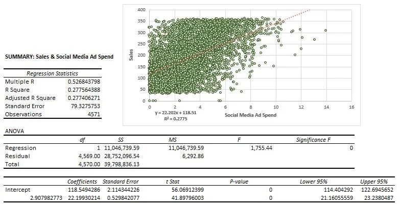
Regression Statistics:
Multiple R: The multiple correlation coefficient (R) indicates the strength and direction of the linear relationship between the independent and dependent variables. In this case, the multiple R value is 0.53, suggesting a moderate positive correlation between the variables.
R Square: 28% of the variability in the dependent variable (sales) can be explained by the independent variable (social media ad spend).
Adjusted R Square: It is very close to the R Square value, indicating that the model is not overfitting. "Not overfitting" implies that the regression model is likely to provide reliable predictions for sales beyond the dataset used to build it.
Standard Error: The standard error of 79.33 indicates the average distance between the observed sales values and the values predicted by the regression model.
Observations: The number of data points used in the regression analysis is 4,571.
ANOVA (Analysis of Variance):
Degrees of Freedom (df), Sum of Squares (SS), & Mean Square (MS): Provide insights into the variability explained by the regression model and the variability left unexplained (residuals). In this case, the large sum of squares for regression relative to the sum of squares for residuals suggests that the regression model explains a significant portion of the variability in sales. This is further supported by the F-statistic and its associated p-value, indicating that the regression model is statistically significant.
F-statistic & Significance F (p-value): (1755.44) with a significance level of 0 indicates that the regression model is statistically significant.
Y-Axis (Dependent Variable - Sales)X-Axis (Independent Variable - Social Media Ad Spend):
Coefficients: The coefficients represent the estimated effects of a one-unit increase in the independent variable (social media ad spend) on the dependent variable (sales). For the Y-axis (sales), the coefficient is 118.55, indicating that for every one-unit increase in social media ad spending, we expect sales to increase by approximately 118.55 units. For the X-axis (social media ad spend), the coefficient is 22.20. This suggests that for every one-unit increase in social media ad spending, sales are expected to increase by approximately 22.20 units.
Standard Errors: Standard errors reflect the precision of the coefficient estimates. For the Y-axis (sales), the standard error is 2.11. This indicates the average amount by which the coefficient may vary from the true value in repeated sampling. For the X-axis (social media ad spend), the standard error is 0.53, suggesting a high precision in estimating the coefficient.
t-Statistics: The t-statistics assess the significance of the coefficient estimates. For the Y-axis (sales), the t-statistic is 56.07, indicating a highly significant relationship between social media ad spend and sales. Similarly, for the X-axis (social media ad spend), the t-statistic is 41.90. This suggests a highly significant relationship.
P-values: P-values represent the probability of observing the t-statistic or more extreme values if the null hypothesis (that the coefficient is equal to zero) is true. For both the Y-axis and X-axis, the p-values are 0, indicating a statistically significant relationship between social media ad spend and sales.
Confidence Intervals: Confidence intervals provide a range of values within which we are confident that the true population coefficient lies. For the Y-axis (sales), the confidence interval ranges from 114.40 to 122.69, while for the X-axis (social media ad spend), it ranges from 21.16 to 23.24. This suggests a high level of certainty in estimating the true effects of social media ad spend on sales.
Summary: Overall, the regression analysis suggests a significant positive relationship between social media ad spending and sales. For every unit increase in social media ad spending, sales are expected to increase by a substantial amount, as indicated by the coefficients. The model explains approximately 28% of the variability in sales, indicating a moderate fit.